Regression Analysis with R


The objective of the report is to analyse the dataset firm-profits and figure out if there is a relation between investment in training and investment in equipment with the amount of profit the company can generate. To understand the impact of investment in training and equipment, we employ econometrics utilizing simple regression analysis and multiple regression analysis while considering other variables which might influence the profits for the company.
Data and Empirical approach
The dataset we analyse has data from 962 firms in it with columns ranging from log_profits, log_training, log_equipment to columns which talk about whether the firm is small or big, if it is an enterprise, if it operates in an industrial sector, if it exports or not, amount of employees it has, age of the firm, whether it does research and development and if they have innovation. After checking and removing abnormal entries, such as values like a million from the Employee_log column in the original dataset, we arrive at the current table with 754 entries (firms) in it.
Our empirical approach derives from the model mentioned below:

In the above equation,
In the above equation, 𝑃𝑟𝑜𝑓𝑖𝑡𝑠𝑖,𝑡 represents profit (in logs) for a firm i in time t = year 2024,
Training𝑖,𝑡−1 & Equipment𝑖,𝑡−1 describe the firm’s investments in training and capital equipment (in logs) during the period 2020 to 2023 (i.e. t-1) respectively,
𝐗′𝑖,𝑡−1 is a vector with other control variables,
𝛼𝑖 is intercept, coefficients 𝛃𝑖(i= 1..x) are the coefficients of interest for each of the variables included as regressors in the model and 𝑢𝑖,𝑡 is the error term.
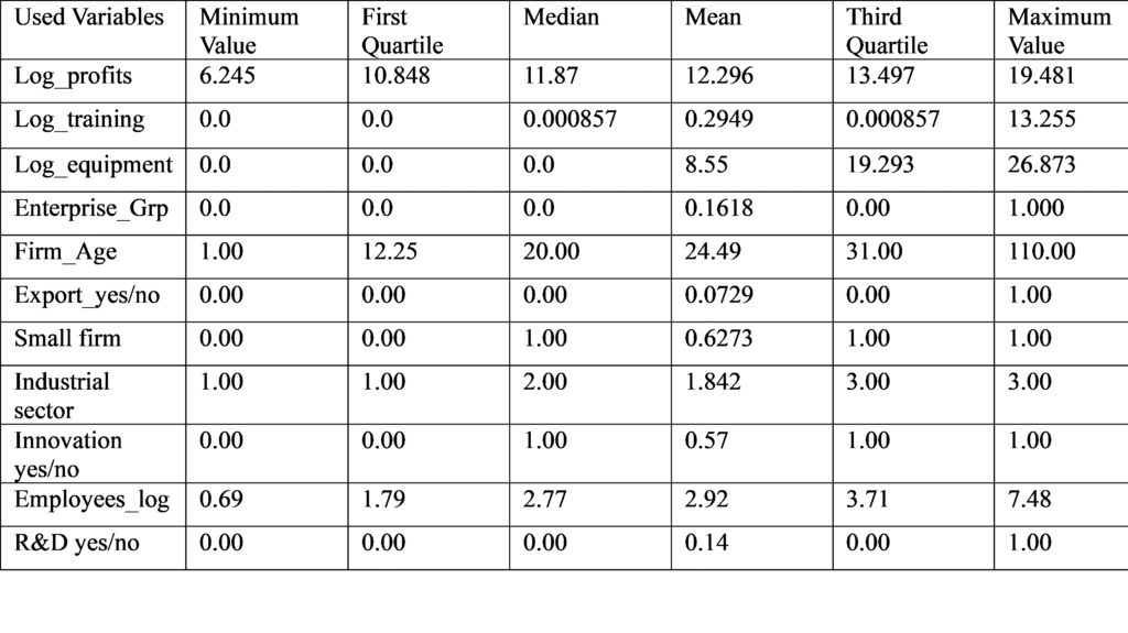
The above table represents the descriptive statistics for the dataset firm-profits. As we can see the age of firms range from minimum at 1 year old to all the way at 110 years old. While most of the firms do not invest in Research and development with their third quartile at 0 and mean at 0.14 in a scale of 0 or 1, the focus on innovation still takes place for at least 50% of the firms with their median at 1 and mean at 0.57 in a similar scale of 0 or 1. The Employees_log ranges from 0.69 all the way to 7.48 showing the firms have a varied range in terms of number of employees.
As for the variable log_profits, values range from minimum at 6.245 to all the way maximum at 19.48 indicating high range of dispersion in profits. The variable profits represent the profitability of the firm. As the data is skewed, with some companies having huge profits while others much lesser than them, the logarithmic scale is used to even out the margin of difference. The log_profits variable has its first quartile at 10.848, meaning 25% of the values in the dataset fall below this mark. The median is at 11.87, meaning 50% of values in the dataset lie below this mark. As for the third quartile, the mark which represents 75% of the values below it, is at the value of 13.497 for the log profits dataset.
For the log training dataset, which represents the investment in training by a firm on a logarithmic scale, both the minimum value and the first quartile is at 0.0. While the mean is at 0.2949, both the median and third quartile is at 0.000857 which showcases that majority of firms have invested next to nothing in training. The same can be interpreted from the scatterplot of log_training vs log_profits.
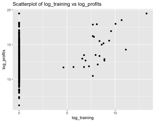
As you can see, in the figure above, log_training for majority of firms is 0 while they still generate profits as represented by log_profits. The few dots on the right side represent the few firms who invested in training and the corresponding profits they generated. The maximum value for log_training is at 13.255 represented by the dot on the farthest right.
For log_equipment, which represents the investment in equipment made by a firm on a logarithmic scale, the minimum value, first quartile and median are all 0. The mean is at 8.55 and third quartile is at 19.29 which means 25% of the firms have invested in equipment at a number more than that. This analysis gets reflected in the scatter plot below between log_profits and log_equipment. While there are a lot of firms which have invested next to nothing in equipment, their firm has still generated profits represented by the dots on Y axis. Although we have to keep in mind, the log_equipment values represent the investment made during the calendar year 2020-2023. In some cases, where the firm_age might be larger, they might have already invested in equipment before 2020 and therefore might not need to invest in it again. For other firms, represents by the dots on the right-hand side in the scatterplot attached below, their investment in equipment have also resulted them in generating profits.
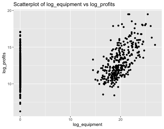
As we can see from the scatter plot, and number of dots represented in the graphs, much more firms have invested in equipment than those who have invested in training.
While scatter plot helps us to analyse basic datapoints, it is very difficult to establish a relationship between log_profits and log_investment or log training, as other factors like age of the firm, number of employees, focus on innovation, which sector the company works in, can play an important role in the determining the profits generated by the company.
To understand more, we employ simple and multiple regression to study the relation between log_profits and log_training, log_investment while also considering other (control) variables as discussed above.
Main Results
As discussed above, to get a better understanding of what effect the different variables have on profits of the firm, we employ different regression models. In the first couple models, we employ simple regression models:
profits= a+b1training+u and profits=a+b1equipment +u.
After that we employ a multiple regression model where profits=a+b1training +b2equipment+u.
After that, we add variables which might influence the profits in the model as well. Lastly, we segregate the small and large firms and observe how the complete model produces separate results for them. The results are encapsulated in the table below.

In the first model, where log_training is the independent variable determining the value of the dependent variable log_profits, value of 𝛃coefficient comes out to be 0.303 which displays a positive relationship between log_training and log_profits while the observation is statistically significant as the p value<0.01. This means that with 1% rise in the value of log_training, there will be a 0.303% rise in the value of log_profits. The value of Rsquare, the coefficient of determination, comes out to be 5.4% which represents the goodness of fit and determines the proportion of variance in the value of log_profits as explained by value of log_training. Also, value of Residual standard error is 1.992, which represents difference between observed values and predicted values, and its low value determines the goodness of the fit of the regression model.
In the second model, where log_equipment is the independent variable determining the value of the dependent variable log_profits, value of 𝛃coefficient comes out to be 0.081 which displays a positive relationship between log_equipment and log_profits while the observation is statistically significant as the p value<0.01. This means that with 1% rise in the value of log_equipment, there will be a 0.081% rise in the value of log_profits. The value of Rsquare, the coefficient of determination, comes out to be 15.6% which means that this model has better fit with respect to the previous model. Also, value of Residual standard error is 1.882, which represents difference between observed values and predicted values, and its low value determines the goodness of the fit of the regression model.
In the third model, where both log_equipment and log_training are used to determine the value of log_profits, value of R square increases to 18.4% showcasing an improvement in the model with better fit. While both independent variables remain statistically significant, 𝛃coefficient for both dips a little owing to the effect they both have on dependent variable, with log_training coefficient at 0.224 with p-value<0.01 and log_equipment coefficient at 0.075 with p-value<0.01. The residual standard error value dips a little at 1.851 displaying improvement in goodness of the fit of the regression model.
For the fourth model, we consider other variables, which might have an impact on the profits generated by a firm. For this, we use the multiple regression model with all the given variables and check the variables with coefficient that are statistically significant, that is their p value<0.05. Apart from log_training and log_equipment, variables such as Enterprise group, Firm Age, Export_yes_no, Small Firm, innovation_yes, R_D_yes, and industrial_sector are the ones which turn out to be statistically significant.
After considering these variables in our multiple regression model, our R square, which signifies the goodness of fit improves substantially and becomes 66.6% signifying that other factors apart from log_training and log_equipment also have a say in driving up the profits for the firm. Also, the value for the residual standard error dips to 1.190 representing a lower value and thus signifying improvement in goodness of the fit of the regression model.
After this, we try and check if our previous model has presence of Heteroskedasticity in it. Generally, the assumption in our regression model is that variance of residual errors is constant i.e. the model is Homoskedastic. We use the studentized Breusch-Pagan test to check if our model is Homoskedastic or not. The BP test produces a test statistic of 30.191 with 9 degrees of freedom and a p-value of 0.000407. As the p-value<0.01, our null hypothesis is rejected, and there is evidence of Heteroskedasticity in the previous model. To counter this, we use a technique called Robust Standard Errors to get more reliable estimates/parameters for our model. After applying robust standard error, while most of the coefficients remain around the same for our fifth model, the F-statistic decreases from 164 to 139 at 9 and 744 degrees of freedom. This means that initial F-statistic was inflated due to presence of heteroskedasticity, and now after applying robust standard error to our fifth model, we have a more reliable estimate.
Next, we divide our dataset into two parts- firms which are small and firms which are large. We apply similar regression analysis as before and create our sixth and seventh regression models based on that. While for small firms, log_training remains significant towards influencing log_profits with a 𝛃coefficient of 0.102 with p value<0.01, large firms do not have log_training variable as a significant factor. Perhaps, this is because is in large firms there is already existing know-how and knowledge gets transferred on the job through colleagues and seniors while small firms specifically require training to advance. On the other hand, while large firms have significant influence from the log_equipment variable towards their profits with a 𝛃coefficient of 0.025 with pvalue<0.01, small firms firms lose log_equipment as a significant factor affecting their log_profits. This can be attributed to the fact that, large firms need continuous investing in equipment to keep producing results and therefore profits, while small firms cannot substantially improve their profits by the presence of investment in equipment alone. Similarly, large firm have Firm_Age as a significant variable but small firms don’t, while Innovation_yes is important for small firms but not for large firms.
Conclusion
I would recommend small firms to invest more in training to improve their profits while saving their extra resources by not spending too much on new and costly equipment. Also, their focus should be on how to innovate to get market attention and attract more funds, thereby providing them with more resources and drive-up profits. While for large firms, they should not waste money on training as knowledge and know-how already exists in the firm and can get transferred through colleagues. Focus for large firms should be on investment in equipment to produce more goods and services they are already producing and thereby improve profits.
Also, they should save their resources and not focus too much on innovation, as they already have an established niche (being a large firm) and should specifically focus on that to improve their profits. Other factors like Exporting goods/services, and having an Enterprise group is important for both small and large firms in improving their profits.
While these conclusions are supported by models as discussed above, our regression analysis suffers from certain limitations. Fact is that our empirical approach assumes a linear relationship between independent and dependent variables. If the relationship is not linear, we might have biased estimates and inaccurate predictions. To fix that we can use polynomial regression. Using too many variables in our regression model might lead to overfitting with the model capturing noise in the data rather than actual existing relationships. To counter that, we can either use Lasso or Ridge regression. Also, there are certain values of the independent variables that might be too influential or prove to be outliers. We can use leverage test alongside cooks’ test to remove influential values. Dividing the original dataset into training and test dataset to further verify these values can improve the robustness of our models.